Toy dataset
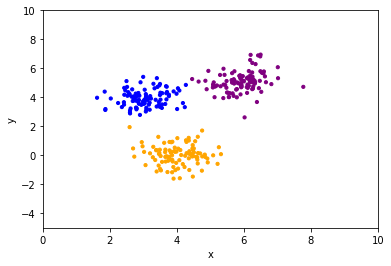
We used here an artificial toy dataset composed of 3 sets of points with 2D random coordinates around an arbitrary center.
To go through this example, you need to install AutoClassWrapper:
$ python3 -m pip install autoclasswrapper
AutoClass C also needs to be installed locally and available in path.
Here is a quick solution for a Linux Bash shell:
wget https://ti.arc.nasa.gov/m/project/autoclass/autoclass-c-3-3-6.tar.gz
tar zxvf autoclass-c-3-3-6.tar.gz
rm -f autoclass-c-3-3-6.tar.gz
export PATH=$PATH:$(pwd)/autoclass-c

# if you use a 64-bit operating system,
# you also need to install the standard 32-bit C libraries:
# sudo apt-get install -y libc6-i386
[1]:
from pathlib import Path
import sys
import time

import matplotlib
import matplotlib.pyplot as plt
from matplotlib.lines import Line2D
import numpy as np
import pandas as pd

%matplotlib inline

print("Python:", sys.version)
print("matplotlib:", matplotlib.__version__)
print("numpy:", np.__version__)
print("pandas:", pd.__version__)

import autoclasswrapper as wrapper
print("AutoClassWrapper:", wrapper.__version__)

version = sys.version_info
if not ((version.major >= 3) and (version.minor >= 6)):
    sys.exit("Need Python>=3.6")
Python: 3.7.1 | packaged by conda-forge | (default, Feb 26 2019, 04:48:14)
[GCC 7.3.0]
matplotlib: 3.0.3
numpy: 1.16.2
pandas: 0.24.1
AutoClassWrapper: 1.4.1
Dataset generation
[2]:
size = 100
sigma = 0.6
x = np.concatenate((np.random.normal(3, sigma, size), np.random.normal(4, sigma, size), np.random.normal(6, sigma, size)))
y = np.concatenate((np.random.normal(4, sigma, size), np.random.normal(0, sigma, size), np.random.normal(5, sigma, size)))
color = ["blue"]*size+["orange"]*size+["purple"]*size
name = ["id{:03d}".format(id) for id in range(size*3)]
df = pd.DataFrame.from_dict({"x":x, "y":y, "color":color})
df.index = name
df.index.name = "name"
df.head()
[2]:
| x | y | color | |
|---|---|---|---|
| name | |||
| id000 | 4.268207 | 4.857065 | blue |
| id001 | 3.079047 | 3.985566 | blue |
| id002 | 3.704671 | 4.374195 | blue |
| id003 | 2.681800 | 3.745056 | blue |
| id004 | 3.012738 | 3.704896 | blue |
[3]:
plt.scatter(df["x"], df["y"], color=df["color"], s=10)
plt.xlabel("x")
plt.ylabel("y")
plt.xlim(0, 10)
plt.ylim(-5, 10);
[4]:
# verify all x are > 0
assert min(df["x"]) > 0
Save x and y in 2 different files (that will be later merged)
[5]:
df["x"].to_csv("demo_real_scalar.tsv", sep="\t", header=True)
df["y"].to_csv("demo_real_location.tsv", sep="\t", header=True)
Step 1 - prepare input files
AutoClass C can handle different types of data:
real scalar: numerical values bounded by 0. Examples: length, weight, age…
real location: numerical values, positive and negative. Examples: position, microarray log ratio, elevation…
discrete: qualitative data. Examples: color, phenotype, name…
Each data type must be entered in separate input file.
AutoClass C handles very well missing data. Missing data must be represented by nothing (no NA, ?, None…)
[6]:
# Create object to prepare dataset.
clust = wrapper.Input()

# Load datasets from tsv files.
clust.add_input_data("demo_real_scalar.tsv", "real scalar")
clust.add_input_data("demo_real_location.tsv", "real location")

# Prepare input data:
# - create a final dataframe
# - merge datasets if multiple inputs
clust.prepare_input_data()

# Create files needed by AutoClass.
clust.create_db2_file()
clust.create_hd2_file()
clust.create_model_file()
clust.create_sparams_file()
clust.create_rparams_file()
2019-07-07 19:07:11 INFO     Reading data file 'demo_real_scalar.tsv' as 'real scalar' with error 0.01
2019-07-07 19:07:11 INFO     Detected encoding: ascii
2019-07-07 19:07:11 INFO     Found 300 rows and 2 columns
2019-07-07 19:07:11 DEBUG    Checking column names
2019-07-07 19:07:11 DEBUG    Index name 'name'
2019-07-07 19:07:11 DEBUG    Column name 'x'
2019-07-07 19:07:11 INFO     Checking data format
2019-07-07 19:07:11 INFO     Column 'x'
2019-07-07 19:07:11 INFO     count    300.000000
2019-07-07 19:07:11 INFO     mean       4.331423
2019-07-07 19:07:11 INFO     std        1.316879
2019-07-07 19:07:11 INFO     min        1.616267
2019-07-07 19:07:11 INFO     50%        4.038210
2019-07-07 19:07:11 INFO     max        7.776609
2019-07-07 19:07:11 INFO     ---
2019-07-07 19:07:11 INFO     Reading data file 'demo_real_location.tsv' as 'real location' with error 0.01
2019-07-07 19:07:11 INFO     Detected encoding: ascii
2019-07-07 19:07:11 INFO     Found 300 rows and 2 columns
2019-07-07 19:07:11 DEBUG    Checking column names
2019-07-07 19:07:11 DEBUG    Index name 'name'
2019-07-07 19:07:11 DEBUG    Column name 'y'
2019-07-07 19:07:11 INFO     Checking data format
2019-07-07 19:07:11 INFO     Column 'y'
2019-07-07 19:07:11 INFO     count    300.000000
2019-07-07 19:07:11 INFO     mean       3.018801
2019-07-07 19:07:11 INFO     std        2.263316
2019-07-07 19:07:11 INFO     min       -1.607160
2019-07-07 19:07:11 INFO     50%        3.882919
2019-07-07 19:07:11 INFO     max        6.949139
2019-07-07 19:07:11 INFO     ---
2019-07-07 19:07:11 INFO     Preparing input data
2019-07-07 19:07:11 INFO     Final dataframe has 300 lines and 3 columns
2019-07-07 19:07:11 INFO     Searching for missing values
2019-07-07 19:07:11 INFO     No missing values found
2019-07-07 19:07:11 INFO     Writing autoclass.db2 file
2019-07-07 19:07:11 INFO     If any, missing values will be encoded as '?'
2019-07-07 19:07:11 DEBUG    Writing autoclass.tsv file [for later use]
2019-07-07 19:07:11 INFO     Writing .hd2 file
2019-07-07 19:07:11 INFO     Writing .model file
2019-07-07 19:07:11 INFO     Writing .s-params file
2019-07-07 19:07:11 INFO     Writing .r-params file
Step 2 - prepare run script & run autoclass
The file autoclass-run-success is created if AutoClass C has run without any issue. Otherwise, the file autoclass-run-failure is created.
[7]:
# Clean previous status file and results if a classification has already been performed.
!rm -f autoclass-run-* *.results-bin

# Search autoclass in path.
wrapper.search_autoclass_in_path()

# Create object to run AutoClass.
run = wrapper.Run()

# Prepare run script.
run.create_run_file()

# Run AutoClass.
run.run()
2019-07-07 19:07:14 INFO     AutoClass C executable found in /home/pierre/.soft/bin/autoclass
2019-07-07 19:07:14 INFO     Writing run file
2019-07-07 19:07:14 INFO     AutoClass C executable found in /home/pierre/.soft/bin/autoclass
2019-07-07 19:07:14 INFO     AutoClass C version: AUTOCLASS C (version 3.3.6unx)
2019-07-07 19:07:14 INFO     Running clustering...
Step 3 - parse and format results
AutoClass C results are parsed and formated for an easier use :
.cdt: cluster data (CDT) files can be open with Java Treeview.tsv: Tab-separated values (TSV) file can be easily open and process with Microsoft Excel, R, Python…_stats.tsv: basic statistics for all classes_dendrogram.png: figure with a dendrogram showing relationship between classes
Note that the \(n\) classes are numbered from 1 to \(n\).
Results are analyzed only when classification is completed.
[8]:
timer = 0
step = 2
while not Path("autoclass-run-success").exists():
    timer += step
    sys.stdout.write("\r")
    sys.stdout.write(f"Time: {timer} sec.")
    sys.stdout.flush()
    time.sleep(step)

results = wrapper.Output()
results.extract_results()
results.aggregate_input_data()
results.write_cdt()
results.write_cdt(with_proba=True)
results.write_class_stats()
results.write_dendrogram()
Time: 2 sec.
2019-07-07 19:07:18 INFO     Extracting autoclass results
2019-07-07 19:07:18 INFO     Found 300 cases classified in 3 classes
2019-07-07 19:07:18 INFO     Aggregating input data
2019-07-07 19:07:18 INFO     Writing classes + probabilities .tsv file
2019-07-07 19:07:18 INFO     Writing .cdt file
2019-07-07 19:07:18 INFO     Writing .cdt file (with probabilities)
2019-07-07 19:07:18 INFO     Writing class statistics
2019-07-07 19:07:18 INFO     Writing dendrogram
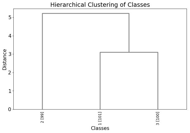
The dendrogram exhibits relationship between classes.
Numbers in brakets are the number of cases (genes, proteins) in a class.
In the above plot, classes 1 and 3 are closer to each other than to class 2. Class 1 has 101 cases, class 3 has 99 and class 2 has 100.
Results exploration
All results are combined in *_out.tsv file.
In addition to the original data (columns name, x and y), the class assigned to a particular case (gene, protein) is given (main-class) along with its probability (main-class-proba). Probability to belong to all classes (class-x-proba) are also provided.
[9]:
df_res = pd.read_csv("autoclass_out.tsv", sep="\t")
df_res.head()
[9]:
| name | x | y | main-class | main-class-proba | class-1-proba | class-2-proba | class-3-proba | |
|---|---|---|---|---|---|---|---|---|
| 0 | id000 | 4.268207 | 4.857065 | 1 | 0.964 | 0.964 | 0.0 | 0.036 |
| 1 | id001 | 3.079047 | 3.985566 | 1 | 1.000 | 1.000 | 0.0 | 0.000 |
| 2 | id002 | 3.704671 | 4.374195 | 1 | 1.000 | 1.000 | 0.0 | 0.000 |
| 3 | id003 | 2.681800 | 3.745056 | 1 | 1.000 | 1.000 | 0.0 | 0.000 |
| 4 | id004 | 3.012738 | 3.704896 | 1 | 1.000 | 1.000 | 0.0 | 0.000 |
[10]:
class_to_color = {1: "green",
                  2: "purple",
                  3: "gray",
                  4: "blue",
                  5: "orange",
                  6: "red"}
df_res["main-class"] = df_res["main-class"].replace(class_to_color)
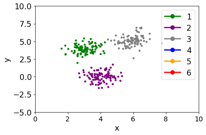
Display classes
[11]:
plt.scatter(df_res["x"], df_res["y"], color=df_res["main-class"], s=10)
plt.xlabel("x")
plt.ylabel("y")
plt.xlim(0, 10)
legend_elements = [Line2D([0], [0], marker='o', color=value, label=str(key), markersize=8)
                   for key, value in class_to_color.items()]
plt.legend(handles=legend_elements)
plt.ylim(-5, 10);
Compare to original distribution
[12]:
plt.scatter(df["x"], df["y"], color=df["color"], s=10)
plt.xlabel("x")
plt.ylabel("y")
plt.xlim(0, 10)
plt.ylim(-5, 10);
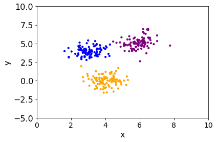
Slight differences could appear at the margin between groups of points but the overall groups are found.